Regression analysis - No26

Today I am going to explain regression analysis.
 Before I talk about analysis method, I would like to start by talking about concept first.
This would be very challenge to me, but I ll try to do my best to explain easily as possible as I can.
I've already mentioned in previous post, regression analysis is focused on causality
between independent variable (response variable) and dependent variable (explanatory variable).
What is this mean ?
In order to answer this question, we can't go further without correlation test.
Once you've tested correlation analysis,
 you can get correlation coefficient value to judge the strength of the relation between two variables.
The correlation coefficient value ranges from -1 to +1 which stands for positive relation or negative trend relation.
 However, this results doesn't explain the exact causality between two variables.
 In other words, By getting the regression coefficient,
we can figure out the ratio of the variability in
independent variable x that affects the explanatory variable y.

Let's assume there are two data sample,
Type 1 shows a positive correlation but Type 2 shows a negative correlation. And
we can get a measureable data which is called  correlation coefficient.
In regression analysis, we use similar index to gauge the strength of correlation.
We called this is  R-squared and this value can get from the square of correlation coefficient.

> cor(Temperature, Discomfort_Index)
[1] 0.9963963
> cor(Temperature, Sales_Long_trousers)
[1] -0.8676816

T-test (two samples)-No25

Today I am going to introduce t-test for two samples.

t-test is a statistical hypothesis test to compare two group.
t-test uses a mean and standard deviation of sample data to determine whether the population means of two group have a relation or not.
Actually, there is an another test which is ANOVA (analysis of variance) has a same purpose. Usually t-test is much more simple than ANOVA test.

This test might be applied in many cases. Such as following
case1) Income gab between city and urban.
case2) New medicine test for patient

Chi-square Test [nonparametric test] -No24

Chi-square test is one of the representative nonparametric test. This test verify the correlation between categorical variables.

In order to verify two discrete variables, chi-square tests statistical differences between observation data and expectations.
This test is also statistical hypothesis test whose null hypothesis is that two categorical variables have no relations.

It is quite easy to understand Chi-square test by conducting a test with different samples.

As you can see below, there are two table which has a data of Candidate preference by man and woman. I would like to compare two data. Intuitively, we can guess that there is no difference by man and woman on case-2. However, there is a quite difference preference on case-1.

Correlaton-No23

Correlation analysis is to measure the correlation between two variables. Important things is this measure just focused on the degree of correlation. but do not explain the exact causality between two values. If you want to get exact causality between the independent variable and dependent variable in given the mathematical equation, you should use the regression test.
There are several types of correlation coefficient to explain correlation.
Today I will focus on the one of the famous tests which is "Pearson correlation coefficient".

This is a value  of the linear correlation range from +1 to -1.
Positive 1 represents strong correlation between two variables. But  negative 1 indicates that two variable is likely to be inversely proportional relation.

Simple Hypothesis Test using R -No22

Today I am going to introduce a hypothesis test using R.
Before moving on to the main test, why don't we review the hypothesis test.
A hypothesis test is a statistical method of decision making which is commonly used.
In order to begin this test, you have to define null hypothesis and alternative hypothesis.

Given the null hypothesis is true, we can figure out the probability and then we make a decision whether we will reject null hypothesis or not. If this probability is really really small, then the result leads us that null hypothesis isn't true.
As a result, we will reject the null hypothesis and favor to alternative hypothesis.
The probability of getting extreme result is called "p-value". Generally,the  decision that whether we should accept null hypothesis or not is depends on our threshold.

As you can see below, I will sample 1,000 data  from the normal distribution which has a standard deviation is 10 and mean is zero.

> data <- rnorm(1000,0,10)

Before we conduct a hypothesis test, we need to define a hypothesis first.
1) Null Hypothesis :  True mean is equal to 0
2) Alternative Hypothesis : True mean is not equal to 0
In fact, we've already know that population mean is 0 because we selected a data from the population distribution whose mean is 0.
Therefore, t-test result should not reject null hypothesis.
Let's look at the test result. This command conducts a test that if the population mean is 0 , in given condition.

Sample Distribution Quiz 2 - No21

Last post, we talked about the way of figuring out the sampling probability from the population distribution.But this time, we will take a look at the method that finds out the population probability using the sample normal distribution.
Most of cases, it is impossible to figure out the population mean. we want to guess the population mean from the sample we got.

I think, this quiz might be happen in your daily lives

Quiz) you sampled 50 students from 3,000 students in your community high schools.
        average height is 150 with a 20 meters sample standard deviation.
        Calculate  the probability  that the average height of all student is
        between 145 and 155.

Sample Distribution Quiz1 - No20

Today I am going to solve a simple quiz based on the knowledge we've learned during last few post.

My quiz is like this.

Can you figure out the probability that sample mean which sampled from the normal distribution (MEAN = 10, SD = 10)  is over 11 ?   (Sample number = 50) 

I emphasized before that we can predict population mean from the sample distribution. however, this is an opposite one because we already know the population mean and standard deviation.

Empirical Rule - No19

This post will guide you how to interpret normal distribution.
We will be able to use normal distribution in order to  predict population mean, so we have to understand the major characteristics of normal distribution.

I think, I already mentioned about "Z score" but today I will explain more about this.
What is Z-Score means ?
Z-score means,  how many standard deviations are away from the mean.
Therefore, Z-score is calculated by below formula.



I explained how to calculate probability in accordance with Z score in post number 16.

Interesting thing is,
As you can see below, there is empirical rule which is very useful to calculate the percentage.

We called this as empirical rule of normal distribution.
If your distribution is normally distributed following rule is applied.
one standard deviation between the mean is occupied 68.2% of the total.
and two stand deviation between the mean is occupied 95.4 of the total.
and third one is occupied 99.6
Someone say this rule is 68.2/95.5/99.6 rule.



[ Normal distribution is defined by   μ = 0 and σ = 1 ]

Inferential analysis basic-2 - No18

I think,  another fundamental concept of inferential analysis is standard error of the mean.
In order to explain this, I am going use same function I used before.

As you can see the  below, the larger your sample number , the smaller  standard deviation. In other words, the shape of your sample distribution of sample mean will become more normal distribution.

Inferential analysis basic-1 - No17

One of the reasons that we are studying inferential analysis is prediction. In some cases, it is impossible to gather whole data to evaluate data character. For example, it is nonsense if you try to check all the products which are produced in your factory to check data quality management. Instead, we take a certain amount of sample and believe the result of evaluation as if  we took all the population.
How does it possible ?
Today I will briefly introduce two major theories make above sample test reliable.

First things is in line with central limit theorem. I think I've already explained overview of central limit theorem in previous post. One thing I didn't clearly prove was average value.
In other words, as you take a mean of sample data over and over again, your sample average will be the  average of population.

I am going to show you by simple test using R.

I've make a new function to get a mean from normal distribution (mean = 5, sd = 10)

Normal distribution - No16

When it comes to the probability distribution, you might be think two distributions.

• Discrete distribution 
• Continuous distribution

Normal distribution is very popular distribution which is a continuous probability distribution defined by below formula.

Central Limit Theorem - No15

I think, central limit theorem is one of the most important theories to understand inferential statistics. Without understanding this, we can't go further for advanced
statistics analysis.

Anyway, I begin to explore the central limit theorem by defining the exact meaning.
There are so many articles to explain this but I chose this excerpt because it is the most appropriate definition for central limit theorem.
The central limit theorem states that, given certain conditions, the mean of a sufficiently large number of independent random variables, each with finite mean and variance, will be approximately normally distributed.  

Before moving on to the next step, it is necessary to pay attention to the important message. In order to guarantee good normal distribution, we have to apply sufficient large number. I ll show you this intuitively using R function.

First, I've prepared a simple function which generates mean from random variables between 1 to 100 s (parent distribution => uniform probability distribution)
And then I'll keep doing this over and over again.

Basic Graph (2) - No14]

This is the second part of basic graph, I am going to introduce different graph.
Some graphs require you to install a specific packages.
New packages can be installed by command (install.packages()) and then you can download a specific package from your favorite mirror site.
In order to use a package function, you have to load package library.

(1)  Scatter plot matrix
First graph I'd like to introduce is scatter plot matrix.
I'll show you two different ways to generate graph.

Scatter plot matrix is useful if your data has a multi variable to compare each other.

* trees data will be used for further test.

> plot(trees)

Basic Graph (1) - No13

When it comes to the R, no doubt, you will be hearing that one of the most powerful functions in R is graphic support. Of course, I feel the same way, too.

Today I will talk about some of R graphic functions and  I will discuss more detail one more time.

I am going to use trees data which is built-in sample data for our demonstration.

> trees

   Girth Height Volume

1    8.3     70   10.3

2    8.6     65   10.3

3    8.8     63   10.2

4   10.5     72   16.4

5   10.7     81   18.8

6   10.8     83   19.7

7   11.0     66   15.6

8   11.0     75   18.2

9   11.1     80   22.6

10  11.2     75   19.9

11  11.3     79   24.2

12  11.4     76   21.0

13  11.4     76   21.4

14  11.7     69   21.3

15  12.0     75   19.1

16  12.9     74   22.2

17  12.9     85   33.8

18  13.3     86   27.4

19  13.7     71   25.7

As you can see, there are three columns. If you want to analyze the relations between

Girth and Volume. 

Standard Deviation- No12

Last two posts, we reviewed the meaning of basic statistics such as qualtile, median, mean etc. Among them, I think average is one of the most common statistics and we use it in our daily lives very often.
For example, math test average score of your class or average height of your class.
However, we can't calculate further meaning with average number.

Let's assume that there are two classes and their mathematics test result are as follows.



>classA <- c( 80, 90, 75, 70, 80, 85. 80)

>classB <- c(100,100,100,100, 55,50,55)

And we can calculate average.

> mean(classA)

[1] 80

> mean(classB)

[1] 80

As you can see, two classes has same average.

Can you tell students of two classes have a similar educational attainment ?

I don't think so because scores of classB are not distributed evenly.

In other words, distance from the average of classB is further than classA.

As a result, I can tell that classA is much more stable than classB in terms of their score.

Data Interpretation(Mean)- No11

Before continuing, review the summary data again.


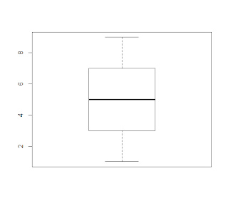
> x <- c(1,2,3,4,5,6,7,8,9)
> summary(x)
   Min. 1st Qu.  Median    Mean 3rd Qu.    Max. 
      1       3         5             5        7             9 


I explained the meaning of quartile last post.
This time, I will explain the box-whisker plot using above information. It is going to be very fun this time because we can learn how to visualize data set so that we can interpret data set more easily.

First, why don't we  focus on the Max, Min result of summary.
Let me skip these two because Minimum or maximum values are commonly used in our daily lives,
Last one is I didn't explain is average.
This is one of the most common statistic and I believe everybody knows about this.
However, average itself is not an appropriate value to judge a measure of dispersion.
I will introduce the meaning of variance and standard deviation next post.

Anyway, I think we are ready to draw a box-whisker plot.
As you can see , bold line in the box one the middle tells you the median value (second qualtile) and this box range between first qualtile and third qualtile.
Lastly, 2 lines connected to dotted line means the maximum and minimum value.

Box and whisker plot is a useful graph to understand whole data set intuitively.

> boxplot(x)

Data Interpretation(Quartile)- No10

In order to have a good insight of the data, I think, we have to enhance an ability to interpret our data. There are so many traditional indexes to interpret our group data such as average, max, standard deviation etc. Furthermore, data can be visualized in diverse graph such as chart graph , bar graph or pie graph.

Fortunately, thanks to great mathematician' achievements, we just need to understand mathematics meaning.

R gives us simple data summaries which has a min,max,median, mean, and qualtile.

Sample result as follows

> x <- c(1,2,3,4,5,6,7,8,9)
> summary(x)
   Min. 1st Qu.  Median    Mean 3rd Qu.    Max. 
      1       3       5       5       7       9 

I will explain mean, median next posts and this post I am going to focus on Qualtiles. 

Making function(2)- No9

Last post we learned how to make your own function. In order to make a complicated function, using control statement is inevitable.

If fact, I already used "for" statement to make a simple function last post.
Today I will introduce two more classic control statement "while" "if"

First let's review the function we made last post.



 Addyourdata <- function (x, N) {
 for (j in 1:N) {
 j=j+1
 x=x+1
 }
 return(x)
 }

Making function(1)- No8

Some people might be think that R is just fabulous scientific calculator but that's wrong.
R is a programming language, you can make your own function or package. Furthermore, if you are a advanced R programmer, you can contribute R package list by submitting and registering your packages to CRAN, then everybody will use your package.

Today I will make a very simple function.
As you are aware, function is a basic unit of R command. you can select and download any packages from CRAN site and then you can use appropriate function for your own purpose.

Let's make a simple scenario.